How to Create a Real-World Project
This guide provides a step-by-step introduction to creating a real-world ViRelAy project from scratch. Building on the foundational knowledge gained through working with the example project in our Example Project article, this tutorial will walk you through the process of designing and implementing a custom classifier and dataset for ViRelAy.
In this guide, we will use a VGG16 model as a concrete example to demonstrate how to create a ViRelAy project. We will train this model on the CIFAR-10 dataset using PyTorch , generate attribution scores for all samples in the dataset using Zennit , and perform an analysis of the data using CoRelAy . The resulting data will be stored in HDF5 databases conforming to the ViRelAy database specification.
Please note that you’re free to substitute these specific model and dataset choices with your own, allowing you to tailor this tutorial to fit your unique requirements and use case.
Prerequisites & Dependencies
Before creating your ViRelAy project, we recommend establishing a virtual environment to isolate dependencies and prevent conflicts with your system’s Python installation. To get started, you’ll need to install some packages that are essential for the project creation process. These dependencies are included as extra dependencies in the ViRelAy package, which can be installed using pip like so:
$ python3 -m venv .venv
$ .venv/bin/pip install 'virelay[examples]'
Accessing the ViRelAy Project Scripts
This guide is accompanied by a set of pre-configured scripts that provide an intuitive command-line interface for creating and managing your ViRelAy project. If you’ve installed ViRelAy from its Git repository, you can find these scripts in the docs/examples directory and the docs/examples/vgg16-project sub-directory.
Alternatively, if you installed ViRelAy using PyPI, you can retrieve the latest version of the VGG16 project scripts from the repository by executing the following commands:
$ mkdir vgg16-project
$ cd vgg16-project
$ curl -o 'meta_analysis.py' 'https://raw.githubusercontent.com/virelay/virelay/main/docs/examples/meta_analysis.py'
$ curl -o 'make_project.py' 'https://raw.githubusercontent.com/virelay/virelay/main/docs/examples/make_project.py'
$ curl -o 'train_vgg.py' 'https://raw.githubusercontent.com/virelay/virelay/main/docs/examples/vgg16-project/train_vgg.py'
$ curl -o 'explain_vgg.py' 'https://raw.githubusercontent.com/virelay/virelay/main/docs/examples/vgg16-project/explain_vgg.py'
$ curl -o 'make_dataset.py' 'https://raw.githubusercontent.com/virelay/virelay/main/docs/examples/vgg16-project/make_dataset.py'
The scripts meta_analysis.py and make_project.py, available under docs/examples , are general-purpose scripts for performing a meta-analysis and creating a ViRelAy project file, which can be used as a starting point for any project. In contrast, the scripts train_vgg.py, explain_vgg.py, and make_dataset.py, available under docs/examples/vgg16-project , are tailored specifically to this VGG16 project but can serve as a blueprint for your own projects. These scripts include:
train_vgg.py– Trains a VGG16 classifier on the CIFAR-10 dataset using PyTorch.explain_vgg.py– Utilizes the trained VGG16 classifier and Zennit to compute attributions for the entire training dataset, storing them in a ViRelAy-compatible database.make_dataset.py– Converts the full CIFAR-10 dataset into a ViRelAy-compatible format.
These scripts provide a solid foundation for creating your own custom projects using ViRelAy.
Training the VGG16 Classifier
As mentioned in the introduction, this guide is based on a VGG16 model trained on CIFAR-10. To create a ViRelAy project from scratch, you’ll need to train the model using the CIFAR-10 dataset. The following code snippet provides an example of how to quickly train the model:
model = vgg16(num_classes=10).to(device)

transform = transforms.Compose([
    transforms.ToTensor(),
    transforms.Normalize((0.4914, 0.4822, 0.4465), (0.2023, 0.1994, 0.2010))
])
train_dataset = CIFAR10(
    root='<dataset-path>',
    train=True,
    download=True,
    transform=transform
)
train_loader = torch.utils.data.DataLoader(train_dataset, batch_size=64, shuffle=True)

loss_function = torch.nn.CrossEntropyLoss()
optimizer = torch.optim.SGD(model.parameters(), lr=0.001, momentum=0.9, weight_decay=5e-4)

for epoch in range(1, 11):
    for batch, labels in train_loader:
        optimizer.zero_grad()
        prediction = model(batch)
        loss = loss_function(prediction, labels)
        loss.backward()
        optimizer.step()

    number_of_correct_predictions = (prediction.argmax(axis=1) == labels).sum().item()
    accuracy = 100 * (number_of_correct_predictions / batch.size(0))
    print(f'Epoch {epoch}, accuracy = {accuracy:.2f}%')

torch.save(model.state_dict(), '<model-path>')
Alternatively, you can use the provided train_vgg.py script to train the VGG16 classifier by executing:
$ .venv/bin/python vgg16-project/train_vgg.py \
    '<dataset-path>' \
    '<model-output-path>' \
    --learning-rate 0.001 \
    --batch-size 64 \
    --number-of-epochs 10
This script trains the model using the specified hyperparameters and saves the trained model to disk at the specified output path.
Project Requirements
A ViRelAy project requires several essential components to function properly. These include:
Dataset – This is the primary input data for your project, which can be stored in either HDF5 format or as an image directory structured by class. The dataset must contain all images that were used to train the classifier.
Label Map – A JSON file that provides a mapping between label indices, class names, and optional WordNet IDs. This file ensures accurate labeling of your data in the ViRelAy user interface.
Attribution Database – An HDF5 file containing attributions computed using a specific attribution method (e.g., using the Zennit framework). Note that each project can only contain attributions for a single method but may have multiple databases per class or other classification categories.
Analysis Database – An HDF5 file holding the results of an analysis pipeline created with CoRelAy. These results include embeddings and clusterings, which can be organized by analysis method, embedding method, or attribution technique.
Project File – A YAML file that ties all other components together, providing metadata about the project.
For a detailed understanding of database and project file structures, please refer to:
These resources provide in-depth information on correctly creating and configuring your ViRelAy project files.
Creating an Attributions Database
Once you have trained a classifier, the next step is to create an attributions database. This process involves organizing the computed attributions, predictions, and ground-truth labels into a structured format.
The structure of the attributions database depends on the shape of your data. If all images have the same size, HDF5 datasets can be used; otherwise, HDF5 groups have to be used. HDF5 datasets are similar to NumPy arrays, i.e., they represent multi-dimensional arrays of data. HDF5 groups on the other hand are more like Python dictionaries, mapping keys to values. For example, in the CIFAR-10 dataset, all images are 32x32 pixels with three color channels, making HDF5 datasets a good choice.
Helper Functions
To simplify the process of creating attribution databases, we provide two helper functions: create_attribution_database and append_attributions. These functions enable you to create an attributions database from scratch and append new attribution data as needed.
def create_attribution_database(
    attribution_database_file_path: str,
    attribution_shape: torch.Size,
    number_of_classes: int,
    number_of_samples: int
) -> h5py.File:

    attribution_database_file = h5py.File(attribution_database_file_path, 'w')
    attribution_database_file.create_dataset(
        'attribution',
        shape=(number_of_samples,) + tuple(attribution_shape),
        dtype=numpy.float32
    )
    attribution_database_file.create_dataset(
        'prediction',
        shape=(number_of_samples, number_of_classes),
        dtype=numpy.float32
    )
    attribution_database_file.create_dataset(
        'label',
        shape=(number_of_samples,),
        dtype=numpy.uint16
    )
    return attribution_database_file

def append_attributions(
    attribution_database_file: str,
    index: int,
    attributions: torch.Tensor,
    predictions: torch.Tensor,
    labels: torch.Tensor
) -> None:

    attribution_database_file['attribution'][index:attributions.shape[0] + index] = (
        attributions.detach().numpy())
    attribution_database_file['prediction'][index:predictions.shape[0] + index] = (
        predictions.detach().numpy())
    attribution_database_file['label'][index:labels.shape[0] + index] = (
        labels.detach().numpy())
The create_attribution_database function initializes an HDF5 file with three datasets:
attribution– Stores the computed attributions.prediction– Holds the predictions of the classifier.label– Contains the ground-truth labels.
The append_attributions function appends new attribution data to the existing database.
Computing Attributions
To compute the attributions, you can use the LRP Epsilon Gamma Box rule with Zennit. This method uses the ZBox rule for the first convolutional layer, the gamma rule for subsequent convolutional layers, and the epsilon rule for fully-connected layers. Please note, that by default, the VGG16 implementation of PyTorch Vision, which is used here, does not use BatchNorm, therefore no canonization is required for LRP to work.
We provide an example code snippet that demonstrates how to cycle through your dataset, compute attributions using the specified rules, and append them to the database.
model = vgg16(num_classes=10)
state_dict = torch.load('<model-path>', map_location='cpu')
model.load_state_dict(state_dict)

transform = transforms.Compose([
    transforms.ToTensor(),
    transforms.Normalize((0.4914, 0.4822, 0.4465), (0.2023, 0.1994, 0.2010))
])
train_dataset = CIFAR10(
    root='<dataset-path>',
    train=True,
    download=True,
    transform=transform
)
train_loader = torch.utils.data.DataLoader(
    train_dataset,
    batch_size=batch_size,
    shuffle=False
)
number_of_samples = len(train_dataset)
number_of_classes = 10

with create_attribution_database(
    '<attribution-database-path>',
    train_dataset[0][0].shape,
    number_of_classes,
    number_of_samples
) as attribution_database_file:

    composite = EpsilonGammaBox(low=-3.0, high=3.0)
    attributor = Gradient(model=model, composite=composite)

    number_of_samples_processed = 0
    with attributor:
        for batch, labels in train_loader:
            predictions, attributions = attributor(
                batch,
                torch.eye(number_of_classes)[labels]
            )
            append_attributions(
                attribution_database_file,
                number_of_samples_processed,
                attributions,
                predictions,
                labels
            )
            number_of_samples_processed += attributions.shape[0]
            print(
                f'Computed {number_of_samples_processed}/{number_of_samples} attributions'
            )
Alternatively, you can use the explain_vgg.py script provided in the VGG16 project directory to train a VGG16 classifier and compute attributions with a single command.
$ .venv/bin/python vgg16-project/explain_vgg.py \
    '<dataset-path>' \
    '<model-path>' \
    '<attribution-database-output-path>'
For more information on how to use Zennit to compute attributions, please refer to the official Zennit documentation .
Converting the Dataset
The CIFAR-10 dataset is provided in a Python pickle format, which is not compatible with ViRelAy. To utilize this dataset within ViRelAy, it must be converted to one of two supported formats: image directories or HDF5 databases.
Image directories store the dataset as separate image files within a directory structure. The top-level dataset directory contains sub-directories for each class, with samples from that class stored in their respective sub-directories. This format is recommended when working with extremely large datasets, where generating a single database file containing the entire dataset would be impractical.
Alternatively, the CIFAR-10 dataset can be stored in an HDF5 database, which offers more efficient storage and faster access times compared to image directories.
Helper Functions
An HDF5 database contains two primary components:
Data – Stores the images themselves as a multi-dimensional array.
Label – Contains the ground-truth labels corresponding to each image.
Depending on whether all images have the same shape, the data and labels can be stored as either HDF5 datasets or HDF5 groups. Given that CIFAR-10 features fixed-size images, HDF5 datasets are employed in this case. To simplify the process of creating and appending samples to an HDF5 database, two convenience functions have been implemented:
def create_dataset(
    dataset_file_path: str,
    samples_shape: torch.Size,
    number_of_samples: int
) -> h5py.File:

    dataset_file = h5py.File(dataset_file_path, 'w')
    dataset_file.create_dataset(
        'data',
        shape=(number_of_samples,) + tuple(samples_shape),
        dtype=numpy.float32
    )
    dataset_file.create_dataset(
        'label',
        shape=(number_of_samples,),
        dtype=numpy.uint16
    )
    return dataset_file

def append_sample(
    dataset_file: h5py.File,
    index: int,
    sample: NDArray[numpy.float64],
    label: NDArray[numpy.float64]
) -> None:

    dataset_file['data'][index] = sample
    dataset_file['label'][index] = label
Additionally, a label map file is required to facilitate the mapping of class indices to human-readable names within ViRelAy. This file can be created using the JSON format, where each entry represents a class and contains its index, WordNet ID, and name.
classes = [
    'Airplane',
    'Automobile',
    'Bird',
    'Cat',
    'Deer',
    'Dog',
    'Frog',
    'Horse',
    'Ship',
    'Truck'
]
wordnet_ids = [
    'n02691156',
    'n02958343',
    'n01503061',
    'n02121620',
    'n02430045',
    'n02084071',
    'n01639765',
    'n02374451',
    'n04194289',
    'n04490091'
]
label_map = [{
    'index': index,
    'word_net_id': wordnet_ids[index],
    'name': classes[index],
} for index in range(number_of_classes)]
with open(label_map_file_path, 'w', encoding='utf-8') as label_map_file:
    json.dump(label_map, label_map_file)
A ready-made script is provided to automate the conversion of the CIFAR-10 dataset into an HDF5 database and generate the corresponding label map file. This script can be executed as follows:
$ .venv/bin/python vgg16-project/make_dataset.py \
    '<dataset-path>' \
    '<dataset-output-path>' \
    '<label-map-output-path>'
Replace <dataset-path>, <dataset-output-path>, and <label-map-output-path> with the actual paths to your dataset, output HDF5 database, and label map file, respectively.
Performing the Meta-Analysis
The meta-analysis phase is a crucial step in creating a ViRelAy project. In this example, we will perform a simple spectral analysis on attributions using CoRelAy, which enables us to construct complex computational pipelines and reuse intermediate results efficiently.
For an introduction to CoRelAy and its capabilities, please refer to the official CoRelAy documentation .
Defining the Analysis Pipeline
The following code listing demonstrates a simple spectral analysis pipeline:
pipeline = SpectralClustering(
    preprocessing=Sequential([
        SumChannel(),
        Normalize(),
        Flatten()
    ]),
    embedding=EigenDecomposition(n_eigval=32, is_output=True),
    clustering=Parallel([
        Parallel([
            KMeans(n_clusters=number_of_clusters) for number_of_clusters in range(2, 31)
        ], broadcast=True),
        TSNEEmbedding()
    ], broadcast=True, is_output=True)
)
This pipeline consists of a preprocessing step, an embedding step using eigenvalue decomposition, and a clustering step using k-Means and t-SNE.
Executing the Analysis Pipeline
The following code listing shows how to execute the analysis pipeline for all categories, i.e., for all classes, in the CIFAR-10 dataset:
with open('<label-map-file-path>', 'r', encoding='utf-8') as label_map_file:
    label_map = json.load(label_map_file)
    wordnet_id_map = {label['index']: label['word_net_id'] for label in label_map}

with h5py.File('<attribution-file-path>', 'r') as attributions_file:
    labels = attributions_file['label'][:]

for class_index in range(10):
    with h5py.File('<attribution-file-path>', 'r') as attributions_file:
        indices_of_samples_in_class, = numpy.nonzero(labels == class_index)
        attribution_data = attributions_file['attribution'][indices_of_samples_in_class, :]

    (eigenvalues, embedding), (kmeans, tsne) = pipeline(attribution_data)

    with h5py.File('<analysis-file-path>', 'w') as analysis_file:

        analysis_name = wordnet_id_map[class_index]

        analysis_group = analysis_file.require_group(analysis_name)
        analysis_group['index'] = indices_of_samples_in_class.astype('uint32')

        embedding_group = analysis_group.require_group('embedding')
        embedding_group['spectral'] = embedding.astype(numpy.float32)
        embedding_group['spectral'].attrs['eigenvalue'] = eigenvalues.astype(numpy.float32)

        embedding_group['tsne'] = tsne.astype(numpy.float32)
        embedding_group['tsne'].attrs['embedding'] = 'spectral'
        embedding_group['tsne'].attrs['index'] = numpy.array([0, 1])

        cluster_group = analysis_group.require_group('cluster')
        for number_of_clusters, clustering in zip(number_of_clusters_list, kmeans):
            clustering_dataset_name = f'kmeans-{number_of_clusters:02d}'
            cluster_group[clustering_dataset_name] = clustering
            cluster_group[clustering_dataset_name].attrs['embedding'] = 'spectral'
            cluster_group[clustering_dataset_name].attrs['k'] = number_of_clusters
            cluster_group[clustering_dataset_name].attrs['index'] = numpy.arange(
                embedding.shape[1],
                dtype=numpy.uint32
            )
This code loads the label map and attribution file, iterates over all classes in the CIFAR-10 dataset, executes the analysis pipeline for each class, and stores the results in an HDF5 analysis database.
Analysis Database Structure
The analysis database is an HDF5 file that contains a group for each category analyzed.Usually, there is one category for each class in the dataset, but the data can be categorized as you wish, e.g., categories can also represent for multiple classes in multi-label classification tasks or other concepts.
Each category group has a key index containing the indices of samples in the category, as well as sub-groups for embeddings and clusterings. The embeddings sub-group contains multiple keys representing different embedding methods, with optional attributes such as eigenvalues and indices. The clusterings sub-group contains multiple keys representing different clustering methods with various parameters.
Usually, there is one category for each class in the dataset, but the data can be categorized as you wish, e.g., categories can be created for multiple classes or even for concepts. For the present project, the data is being categorized by the classes of the CIFAR-10 dataset. Each of the category HDF5 groups of this analysis database will use the WordNet ID of the class as its name (which, again, is just a convention, but if the category name is a WordNet ID, ViRelAy will automatically display the class label). The category groups have a key index, which contains the indices of the samples that are in the category. Furthermore they have sub-group called embedding and a sub-group called cluster, which contain the embeddings and clusterings computed in the analysis pipeline respectively. Each key in the embedding sub-group represents a different embedding method, in this project, the attributions will be embedded using spectral embedding and t-SNE. Each embedding can optionally have multiple attributes: eigenvalue, which contains the eigenvalues of the eigendecomposition of the embedding, embedding, which is the name of the base embedding, if the embedding is based on another embedding, and index, which are the indices of the dimensions of the base embedding that were used. Finally, the cluster sub-group contains the clusterings that were used to cluster the attributions. Each key in the cluster sub-group represents a different clustering method with different parameters. In the case of this project, there is only a k-means clustering for k’s between 2 and 30, so a key for each of these clusterings is generated. Each clustering can have attributes, e.g., embedding, which is the embedding that the clustering is based on, or the parameters of the clustering algorithm.
Running a More Elaborate Analysis Pipeline
To execute a more complex analysis pipeline with additional embedding and clustering methods, use the meta_analysis.py script:
$ .venv/bin/python vgg16-project/meta_analysis.py \
    '<attribution-path>' \
    '<analysis-output-path>' \
    --label-map-file-path '<label-map-path>'
This script takes the attribution path, analysis output path, and label map file path as arguments and runs the meta-analysis pipeline accordingly.
Creating the Project File
Now, we have all the necessary files to create a project: the dataset HDF5 file, the label map JSON file, the attribution HDF5 file, and the analysis HDF5 file. The only thing that is missing now is the project YAML file.
project:
    name: VGG16 CIFAR-10
    model: VGG16
    label_map: <label-map-path>
    dataset:
        name: CIFAR-10
        type: hdf5
        path: <dataset-path>
        input_width: 32
        input_height: 32
        up_sampling_method: none
        down_sampling_method: none
    attributions:
        attribution_method: LRP Epsilon Gamma Box
        attribution_strategy: true_label
        sources:
        - <attribution-path>
    analyses:
    - analysis_method: Spectral
      sources:
      - <analysis-path>
The project YAML file consists of a project name, a model name, a reference to the dataset file, a reference to the label map file, a reference to the attribution files, and a reference to the analysis files. The project and model name can be chosen arbitrarily and are only used to display them, when the project is opened in ViRelAy. These make it easier to distinguish between multiple loaded projects. The dataset requires some more information. The dataset name, again, can be chosen arbitrarily and is only used for informational purposes. The type property is used to distinguish between image directory datasets and datasets that are stored in HDF5 files. The path either represents the path to the image directory or to the HDF5 dataset file. All paths in the project file are relative to the project file itself. The input width and height properties determine the width and height to which the images have to be re-sampled before feeding them into the classifier. In the case of our VGG16 model this is 32x32 pixels. When the images do not all have the same width and height or when the classifier expects a different input size, then the up-sampling and down-sampling methods determine how the images are scaled up when they are too small or how they are scaled down when they are too large, respectively. The label map represents the path to the label map JSON file. The attributions property consist of an attribution method, which is the algorithm that was used to compute the attributions, the attribution strategy, which determines whether the attribution was computed for the true label or the label assigned by the classifier, and a list of source files. This means that the attributions can be split among multiple HDF5 databases, e.g., an attribution file could be created per class. Finally, the analyses property is a list of analyses that were performed on the data. Multiple analyses can be created to compare different analysis methods. Each analysis consists of the name of the analysis method and a list of source files. So each project can have multiple analyses and each analysis can consist of multiple analysis databases. For example, an analysis database could be created per embedding or attribution method.
This file can also be generated by executing the make_project.py script, which can be invoked like so:
$ .venv/bin/python vgg16-project/make_project.py \
    '<dataset-path>' \
    '<attribution-path>' \
    '<analysis-path>' \
    '<label-map-path>' \
    --project-name 'VGG16 CIFAR-10' \
    --dataset-name 'CIFAR-10' \
    --model-name 'VGG16' \
    --attribution-name 'LRP Epsilon Gamma Box' \
    --analysis-name 'Spectral' \
    --output-file-path '<project-output-path>'
When opening the project, created in this guide, in ViRelAy, you will be greeted with a setup like in Figure 1.
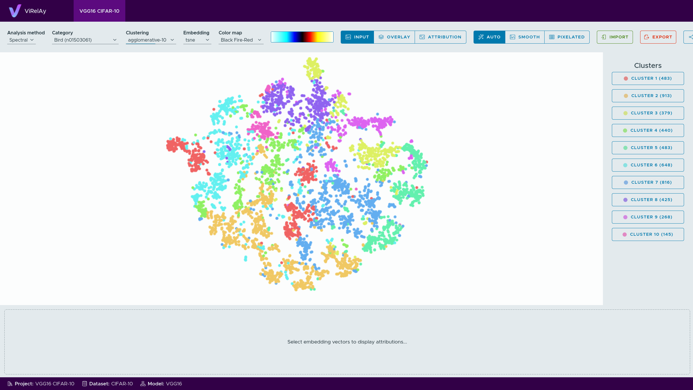
Figure 1: The VGG16 CIFAR-10 project opened in ViRelAy.